Excel Tips - Tip 23 (Using Hyperlink in excel)

Hi Everyone,

Here is the Twenty Third Tip for you. Hope this help you.

How the Hyperlink between the sheets helps us.

It means as you click on the cell, you directly move to that sheet which helps your valuable time. It helps in making Index, Table etc.

How to Use Hyperlink between the sheets.

1. Type the text in the cell

2. Go to the cell in which you want to get hyperlink with the corresponding sheet

3. Go to INSERT tab, and select HYPERLINK from there. Or use shortcut (Alt+N+I)

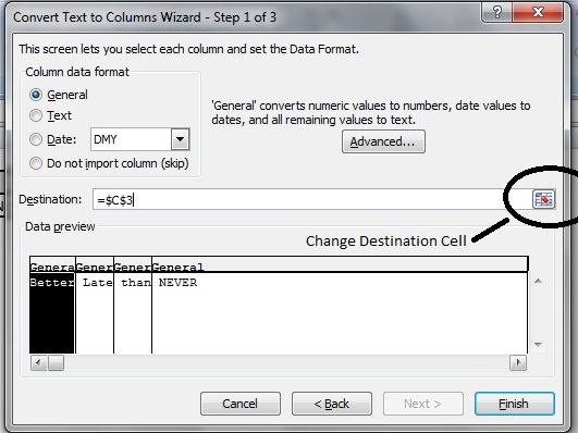
 4. From the dialog box Select Place in this document.

5. Select the Respective sheet from there.

6. Now the cell is hyperlink.

7. Click on the same hyperlinked cell, as you click you will directly go to the that linked sheet.

8. To go back to the hyperlinked cell, Press “F5” in the Hyperlinked sheet. You will come back to the hyperlinked cell.

Hope, this tip is clear with my explanation.

In case of any doubt, please feel free to contact me any time.

If any of your friends is also interested for the said excel Tips, then asked them to fill the form by clicking on the below mentioned link:

https://docs.google.com/forms/d/12T8v5XY0XlF9IhuCZPQpydd8hjCtrW7hZs9_GiOffIw/viewform?c=0&w=1

If you have something that you want to share with the group, please write to excelms.tips@gmail.com

Please do share your valuable feedback. Keep Sharing.

Thanks & Regards,

CA Mohit Bansal

Excel Enthusiast

+91-9045773456

Excel Tips - Tip 22 (Using Wrap Text)

Hi Everyone,

Here is the Twenty second Tip for you.  Hope this help you.

Whenever you type the Text in a Cell which is more than the width of the cell, then you have option of Merge.

Here is an alternative of the merge.

You can use “Wrap Text” on the selected cell. It will help you in restricting your text in the width of the text.

 Shortcut key of the same (Alt+H+W) or Go to Home and then select Wrap Text from there.

Hope, this tip is clear with my explanation. In case of any doubt, please feel free to contact me any time.

If any of your friends is also interested for the said excel Tips, then asked them to fill the form by clicking on the below mentioned link:

https://docs.google.com/forms/d/12T8v5XY0XlF9IhuCZPQpydd8hjCtrW7hZs9_GiOffIw/viewform?c=0&w=1

If you have something that you want to share with the group, please write to excelms.tips@gmail.com

Please do share your valuable feedback. Keep Sharing.

Thanks & Regards,

CA Mohit Bansal

Excel Enthusiast

+91-9045773456

Excel Tips - Tip 21 (Show all Formulaes)

Hello Everyone,

Here is the Twenty First Tip for you.

Today's excel tip is about displaying formulas in excel.

All of you know that you can display a formula by pressing F2 in the relevant cell or you can view the formula in the formula bar.

But what if you want all the formulas to be displayed at once.

I mean all the formulas in the workbook.........

You can do this by pressing Ctrl and `.

To restore press the same combination again

Note - ` key is usually found on the key to the left of number 1.

Hope, this tip is clear with my explanation.

In case of any doubt, please feel free to contact me any time.

If any of your friends is also interested for the said excel Tips, then asked them to fill the form by clicking on the below mentioned link:

https://docs.google.com/forms/d/12T8v5XY0XlF9IhuCZPQpydd8hjCtrW7hZs9_GiOffIw/viewform?c=0&w=1

If you have something that you want to share with the group, please write to excelms.tips@gmail.com

Please do share your valuable feedback. Keep Sharing.

Thanks & Regards,

CA Mohit Bansal

Excel Enthusiast

 +91-9045773456

Excel Tips - Tip 20 (Using Data Validation)

Hi Everyone,

Here is the Twentieth tip for you. Hope this help you.

Ever wanted to restrict data entry in certain cells to a limited set of vales??

Here is how you can use data validation feature in MS Excel.

What does it do??

Creating drop-down list and enforcing data entry using drop-down, ensures that data consistency is always maintained in your worksheet.

How to use it ??

1. Enter the list of items in a range.

2. Select the cell that will contain the drop-down list

3. Choose Data -> Data Tools -> Data Validation.

4. In the Data Validation dialog box, click the Settings tab.

5. In the Allow drop-down list, select List.

6. In the Source box, specify the range that contains the items.

7. Make sure that the In-Cell drop-down option is checked and click OK.

Bonus Tip: If the drop-down list is short, then you can enter the values directly in the Source Field separated by commas.

In Case you type the wrong data, then an error will show as shown in images.

Hope, this tip is clear with my explanation.

In case of any doubt, please feel free to contact me any time.

If any of your friends is also interested for the said excel Tips, then asked them to fill the form by clicking on the below mentioned link:

https://docs.google.com/forms/d/12T8v5XY0XlF9IhuCZPQpydd8hjCtrW7hZs9_GiOffIw/viewform?c=0&w=1

If you have something that you want to share with the group, please write to excelms.tips@gmail.com

Please do share your valuable feedback. Keep Sharing.

Thanks & Regards,

CA Mohit Bansal

Excel Enthusiast

 +91-9045773456

Excel Tips - Tip 19 (Remove and Highlight Duplicate Values)

Hello,

Here is the Nineteenth tip for you. Hope this help you.

Using shortcut command to Highlight Duplicate values and Removing Duplicate Values will surely ease your working and save your valuable time.

How to Remove Duplicates Values?

1. Select the data in which you want to Remove the Duplicate Values

2. Press (Alt+A +M) or Go to “Data Tab” and then click on “Remove Duplicate” icon.

3. A dialog box will appear as soon as you complete the Step 2. As shown in Images attached.

4. Select continue with Current Selection, if you don’t want to loose your data in another column.

5. Press Enter, after choosing the desired option.

6. All duplicate Values are removed from the said column.

How to Highlight Duplicates Values?

1. Select the data in which you want to Highlight the Duplicate Values

2. Press (Alt+H+L+H+D) or Go to “Home Tab” and then click on “Conditional Formatting” icon and from there choose “Highlight Cells Rules” and click on duplicate values.

3. A dialog box will appear as soon as you complete the Step 2. As shown in Attached Images

4. Press Enter, and the duplicate values are Highlighted

Hope, this tip is clear with my explanation.

In case of any doubt, please feel free to contact me any time.

If any of your friends is also interested for the said excel Tips, then asked them to fill the form by clicking on the below mentioned link:

https://docs.google.com/forms/d/12T8v5XY0XlF9IhuCZPQpydd8hjCtrW7hZs9_GiOffIw/viewform?c=0&w=1

If you have something that you want to share with the group, please write to excelms.tips@gmail.com

Please do share your valuable feedback. Keep Sharing.

Thanks & Regards,

CA Mohit Bansal

Excel Enthusiast

+91-9045773456

Excel Tips - Tip 18 (Using Text to Column Formulae )

Hello,

After all the appreciation and positive feedback, I am pleased to continue my tips.

Here is the Eighteenth tip for you. Hope this help you.

Using Text to Column is very easy and effective.

Hope it will help you in ease your work.

How it work?

1. Select the cell where you want to split the text into different cells

2. Use shortcut Key (Alt+A+E), alternatively you can go to Data Tab and Select “Text to columns” from the drop down menu.

3. A dialog box will appear as shown in below image.

4. Here you have an option to select “Delimited” or “Fixed” option.

5. In “Delimited” you have pre defined instructions like “Tab “, “Semicolon”, “Comma”, “Space” as shown in figure.

6. In “Fixed” you can scale the split text according to your need by moving the Scale in “Data Preview”.

7. After selecting the option, Click “Next”

8. As soon As you click on Next, A preview of your data is shown in table as shown in figure.

9. If you are satisfied with the preview, then click on “Next” Button,

10. Now the Dialog box will ask you about the “Destination Cell” of your spited text. Select the desired cell.

11. Now Click on “Finish”

12. Result- Your text is spitted into different cells.

Here are the example of above command with dialog box Images.

Hope, this tip is clear with my explanation.

In case of any doubt, please feel free to contact me any time.

If any of your friends is also interested for the said excel Tips, then asked them to fill the form by clicking on the below mentioned link:

 https://docs.google.com/forms/d/12T8v5XY0XlF9IhuCZPQpydd8hjCtrW7hZs9_GiOffIw/viewform?c=0&w=1

If you have something that you want to share with the group, please write to excelms.tips@gmail.com

Please do share your valuable feedback. Keep Sharing.

Thanks & Regards,

CA Mohit Bansal

Excel Enthusiast

+91-9045773456